Monetary Policy and Aggregate Demand

Week 05

Vivaldo Mendes

vivaldo.mendes@iscte-iul.pt

Instituto Universitário de Lisboa (ISCTE-IUL)

March 10, 2025

Recall: The Fisher Equation

In Week 2 we discussed a very important concept: the Fisher Equation \[ r=i-\pi \] \(i:\) \(~\)nominal interest rate ; \(~~\) \(r:\) \(~\) real interest rate ; \(~~\) \(\pi:\) \(~\) rate of inflation
In the short-term, from one day to the other, the Fed can change its short-term interest rate \((i)\).
But prices are sticky (rigid); they take time to change given new circumstances. So, \(\pi\) is rigid in the short-term.
Therefore, the Fed can affect the real interest rate \((r)\) in the short-term, when it announces a change in its (nominal) rates.

1. The Monetary Policy Curve (MP)

The Fed and the FFR

It is useful to highlight some acronyms:

Fed: Federal Reserve Board (the central of the USA)
FFR : Federal Funds Rate
- The overnight interest rate that commercial banks charge each other when lending amounts of funds (also called reserves) in a uncollateralized basis
Target rate range: the range set by the Fed (by law) for the short term interest rate
Volume of trade: the amounts of uncollateralized funds (reserves) that are traded between commercial banks in everyday

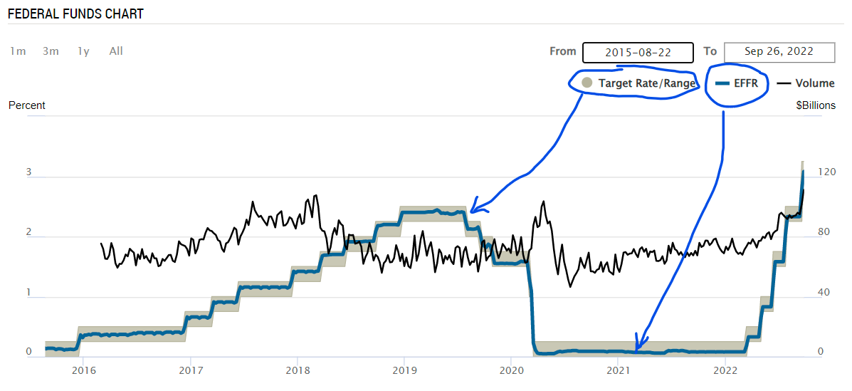
The Fed and the FFR

A single image obtained from Fed New York shows all in a simple way:

The Monetary Policy Curve (MP)

The Fed bases its decisions to change short term interest rates on 3 factors:
- The natural real interest rate: \((\bar{r})\)¹
- The rate of inflation: \((\pi)\)
- The output gap: \((realGDP - PotentialGDP)\)
To simplify the exposition, the textbook avoids the output-gap impact on the Fed’s decision making process until later chapters.
So, the simple version of the monetary policy rule (MP) is: \[ r=\bar{r}+\lambda \pi \tag{1} \]
\(\lambda\) is a parameter and tells how much the central bank dislikes inflation.

The MP Curve: Graphical Representation

The MP curve is given by: \(\quad r=\overline{r}+\lambda \pi\)

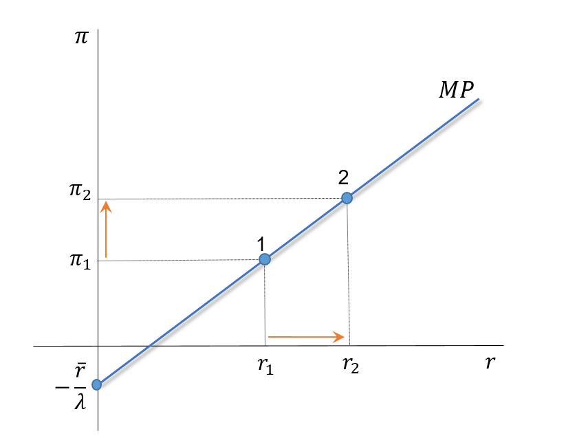
From point 1 to 2:

As inflation raises from \(\pi_1\) to \(\pi_2\)
The Fed is forced to increase real interest rates from \(r_1\) to \(r_2\).
\(\Delta \overline{r}=0\)
If \(\Delta \overline{r} \neq 0\), the curve shifts

The Taylor Principle

Definition. The Taylor principle

The Taylor principle states that to avoid inflationary spirals—inflation that gets higher and higher over time—the central bank must increase the nominal interest rate by more than the change in the inflation rate.

The Taylor principle will be satisfied when \[\lambda>0\]
If \(\ \lambda>0 \ \Rightarrow \ \Delta i > \Delta \pi \ \) always

The Taylor Principle: An Example

Suppose that: \(\lambda = 0.5 \ \ ; \ \Delta \pi = +1pp\)
From the MP curve: \[\Delta r=\Delta \bar{r}+\lambda \times \Delta \pi=0+0.5 \times 1=0.5\]
From the Fisher equation: \[\Delta r=\Delta i-\Delta \pi \Rightarrow \Delta i=1+0.5=1.5\]
So, we have: \(\Delta i=1.5>\Delta \pi=1\)
The increase in inflation will be controlled: \[\pi \ \uparrow \ \Rightarrow \ r \ \uparrow \ \Rightarrow \ Y \ \downarrow \ \Rightarrow \ \pi \ \downarrow \ \Rightarrow \ \text{inflation is controled}\]
Otherwise, we would end up in an inflationary spiral: \[ \pi \ \uparrow \ \Rightarrow \ r \ \downarrow \ \Rightarrow \ Y \ \uparrow \ \Rightarrow \ \pi \ \uparrow \ \Rightarrow \ r \ \downarrow \ \Rightarrow \ Y \ \uparrow \ \Rightarrow \ \pi \ \uparrow \ldots \]

MP Curve: Shifts

The MP curve is given by: \(\quad r=\overline{r}+\lambda \pi\)

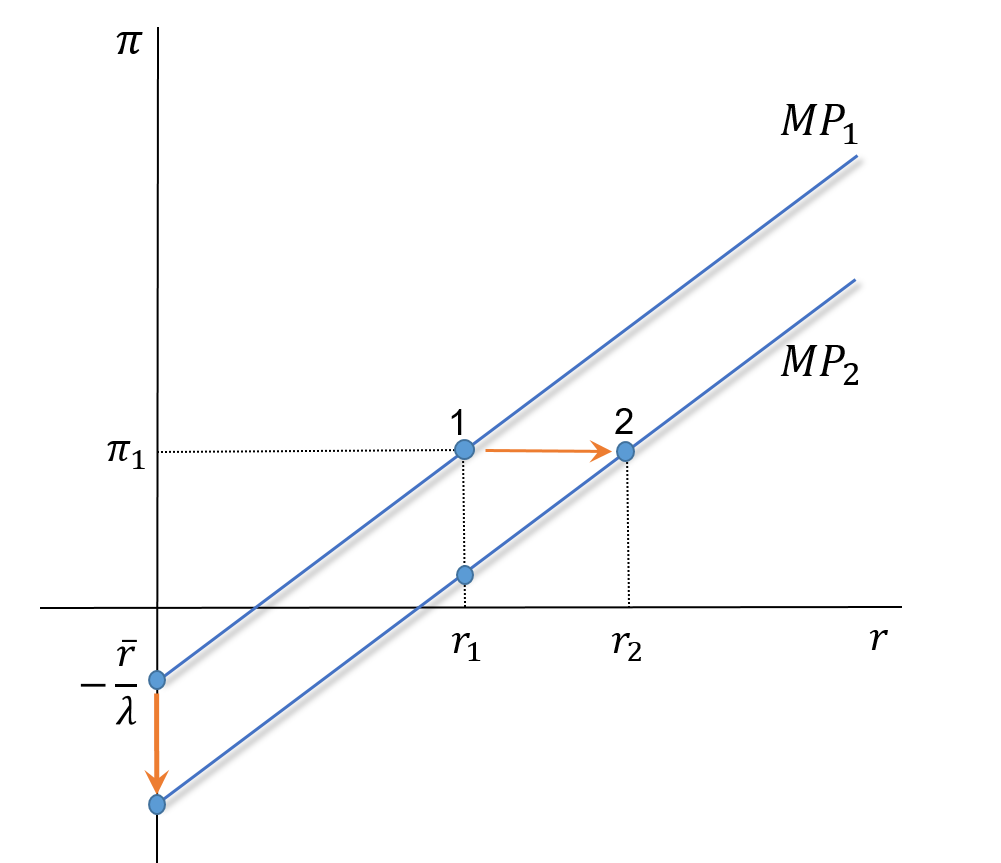
From point 1 to 2:

If \(\bar{r}\) increases, the MP curve shifts to the right, and vice-versa.
Notice that \(r\) increases, but \(\pi\) remains constant.

Policy and Practice

There are two types of reaction by the central bank:

An accommodating monetary policy (movement along the MP curve)
An aggressive monetary policy (a shift in the MP curve)

Policy and Practice

In the figure below, can we distinguish between those two reactions? Why one? Why the other?

2. The Aggregate Demand Curve (AD)

The Logic Behind the AD Curve

The MP curve demonstrates how central banks respond to changes in inflation with changes in interest rates, in line with the Taylor principle.
The IS curve we developed in Week 4 showed that changes in interest rates, in turn, affect GDP.
Using these two curves, we can link the level of GDPe to the level of the inflation rate.
In a simple way: \[ M P=I S \rightarrow A D \]

Derivation of the AD Curve

Recall the IS curve \[ Y=m \cdot \bar{A}-m \cdot \phi \cdot r \tag{2} \]

Now the MP curve: \[ r=\bar{r}+\lambda \cdot \pi \tag{3} \]

Insert eq. (3) into eq. (2), and we get the AD curve: \[ Y=m \cdot \bar{A}-m \cdot \phi \cdot(\bar{r}+\lambda \pi) \tag{4} \]

AD Curve: Graphical Representation

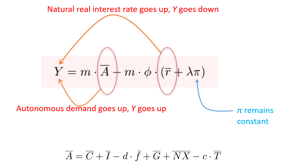
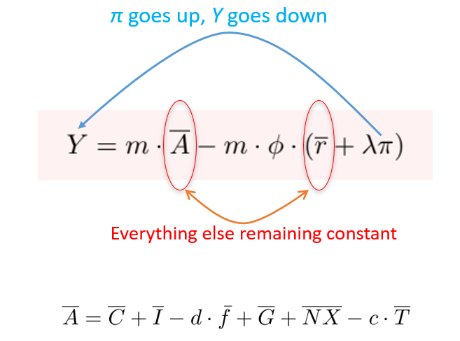
The AD curve is given by: \(\quad Y=m \cdot \bar{A}-m \cdot \phi \cdot(\bar{r}+\lambda \pi)\)

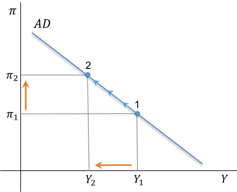
From point 1 to 2:

If \(\pi\) increases, the central bank will raise \(i\) and \(r\)
As \(i\) and \(r\) go up, demand will go down, and GDP will follow.
This occurs if \(\Delta \overline{A}=0\)

AD Curve: A Shift

The AD curve is given by: \(\quad Y=m \cdot \bar{A}-m \cdot \phi \cdot(\bar{r}+\lambda \pi)\)

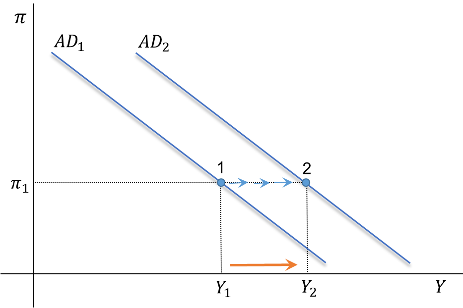
From point 1 to 2:

If \(\pi\) remains constant, the central bank will keep \(i\) and \(r\) constant.
If those rates are constant, and \(\Delta \overline{A}>0\), then demand and GDP go up.

3. AD Curve: Summary

A Movement Along the AD Curve

A Shift of the AD Curve

4. Readings

Readings

Read Chapter 10 of the adopted textbook:

Frederic S. Mishkin (2015). Macroeconomics: Policy & Practice, Second Edition, Pearson Editors

Two important notes:

Do not study the graphical analysis in Figures 10.4, 10.5, and 10.6 in the chaper above. These slides simplify the graphical analysis presented in this chapter of the textbook a lot. Those figures do not add any significant point to the presentation and will take up too much of your time.
The section “The Money Market and Interest Rates” in the chapter above, which starts on page 263, will be postponed to next week’s materials.